Module 2: Spatial Jacobian and Resolved-Rate Trajectories
This module has two parts. Part A computes the spatial manipulator Jacobian \( J_s \) of the UR5e using the twists from Module 1, and checks it against the velocity sensors mounted on the robot’s wrist. Part B uses that Jacobian to move the wrist along a straight-line path with resolved-rate trajectory generation, and compares it against a straight line in joint space.
Complete Module 1 first. This module uses your
joint_twistsandforward_kinematics_exponentialfunctions.
By the end of this module, your folder should look like this:
ur5e/
  ur5e_model/          UR5e model, from setting up
  transforms.py        helper functions (from Module 1)
  kinematics.py        your kinematics (add two functions in Part A)
  trajectories.py      your trajectory code (Part B, fill in the TODOs)
  module1.py           (from Module 1)
  module2_jacobian.py  runs the Part A simulation (copy as-is)
  module2_path.py      runs the Part B simulation (copy as-is)
The UR5e motors in this model are position servos: the scripts in this module set
d.ctrlto the desired joint angles, and each motor applies a torque based on the error between the desired and actual angle.
Part A: Spatial Jacobian
Background
Each column of the spatial Jacobian is the twist of joint \( i \), moved to the robot’s current configuration:
\[J_s(\theta) = \begin{bmatrix} \xi'_1 & \xi'_2 & \cdots & \xi'_6 \end{bmatrix}, \qquad \xi'_i = \mathrm{Ad}_{\,e^{\hat{\xi}_1 \theta_1} \cdots e^{\hat{\xi}_{i-1} \theta_{i-1}}} \, \xi_i ,\]where \( \xi_i \) are the same twists you found for the product of exponentials in Module 1. For a twist \( \xi = (v, \omega) \), the adjoint of \( g = (R, p) \) is the \( 6 \times 6 \) matrix
\[\mathrm{Ad}_g = \begin{bmatrix} R & [p]_\times R \\ 0 & R \end{bmatrix}.\]Skeleton Code
Add the following to the bottom of your kinematics.py. Your job is to fill in the parts marked TODO.
from transforms import skew


def adjoint(g):
    """6x6 adjoint of the 4x4 homogeneous transformation g, for twists [v; omega]."""
    R = g[:3, :3]
    p = g[:3, 3]
    # TODO: build the adjoint from R and p
    return np.zeros((6, 6))


def spatial_jacobian(theta):
    twists = joint_twists()
    Js = np.zeros((6, 6))
    g = np.eye(4)  # product of the exponentials of the joints before joint i
    for i in range(6):
        # TODO: column i of the spatial Jacobian
        Js[:, i] = np.zeros(6)

        g = g @ expm(twist_matrix(twists[i]) * theta[i])
    return Js
Running/Testing your Code
Create module2_jacobian.py with the following content. The arm swings each joint back and forth for six seconds while the script compares two spatial twists of the wrist:
- \( J_s \dot{\theta} \), from your Jacobian and the joint velocities, and
- the twist measured by a velocimeter and gyroscope at the wrist. These sensors measure the body twist \( \xi_b \), which the script converts to the spatial twist using \( \xi_s = \mathrm{Ad}_{g} \, \xi_b \). The wrist pose \( g \) used here comes from MuJoCo, not from your code.
import time
import mujoco
import mujoco.viewer
import numpy as np
import matplotlib
matplotlib.use("Agg")  # save the plot to a file instead of opening a window
import matplotlib.pyplot as plt
from transforms import homogeneous
from kinematics import spatial_jacobian, adjoint

m = mujoco.MjModel.from_xml_path("ur5e_model/scene.xml")
d = mujoco.MjData(m)
wrist = m.site("wrist").id

# A smooth joint motion for the arm to follow: each joint swings back and forth
q_center = np.array([0, -np.pi/2, np.pi/2, -np.pi/2, -np.pi/2, 0])
amplitude = np.array([0.6, 0.4, 0.5, 0.6, 0.6, 0.8])
frequency = np.array([0.20, 0.25, 0.30, 0.35, 0.40, 0.45])  # Hz
duration = 6.0  # seconds

def q_desired(t):
    return q_center + amplitude * np.sin(2 * np.pi * frequency * t)

d.qpos[:6] = q_desired(0)
times, xi_jacobian, xi_sensor = [], [], []

with mujoco.viewer.launch_passive(m, d) as viewer:
    while viewer.is_running() and d.time < duration:
        step_start = time.time()

        # The UR5e motors are position servos: d.ctrl is the desired joint angle
        d.ctrl[:] = q_desired(d.time)
        mujoco.mj_step(m, d)
        mujoco.mj_forward(m, d)  # update the sensors to the new joint angles and velocities

        # Spatial twist from your Jacobian
        xi_J = spatial_jacobian(d.qpos[:6]) @ d.qvel[:6]

        # Spatial twist from the sensors at the wrist. The velocimeter and gyro
        # measure the body twist, which the adjoint of the wrist pose (from
        # MuJoCo, not your code) converts to the spatial twist.
        g_wrist = homogeneous(d.site_xmat[wrist].reshape(3, 3), d.site_xpos[wrist])
        xi_S = adjoint(g_wrist) @ d.sensordata[:6]

        times.append(d.time)
        xi_jacobian.append(xi_J)
        xi_sensor.append(xi_S)

        viewer.sync()
        time.sleep(max(0, m.opt.timestep - (time.time() - step_start)))

# Plot the six components of both spatial twists
xi_jacobian, xi_sensor = np.array(xi_jacobian), np.array(xi_sensor)
labels = ["$v_x$ (m/s)", "$v_y$ (m/s)", "$v_z$ (m/s)",
          r"$\omega_x$ (rad/s)", r"$\omega_y$ (rad/s)", r"$\omega_z$ (rad/s)"]
fig, axs = plt.subplots(2, 3, figsize=(14, 7), sharex=True)
for i, ax in enumerate(axs.flat):
    ax.plot(times, xi_sensor[:, i], linewidth=3, label="Sensors")
    ax.plot(times, xi_jacobian[:, i], "--", linewidth=2, label="$J_s \\dot{\\theta}$")
    ax.set_ylabel(labels[i])
    ax.grid(True)
for ax in axs[1]:
    ax.set_xlabel("Time (s)")
axs[0, 0].legend()
fig.tight_layout()
fig.savefig("module2_twist.png", dpi=150)
print("Largest difference:", np.abs(xi_jacobian - xi_sensor).max())
print("Saved module2_twist.png")
Then run it from your folder:
python module2_jacobian.py
macOS: use
mjpythoninstead ofpythonto run any script that opens the viewer, e.g.mjpython module2_jacobian.py.
When the motion ends, the script saves the plot module2_twist.png and prints the largest difference between the two twists. If your Jacobian is correct, the lines overlap in all six plots and the printed difference is close to zero:
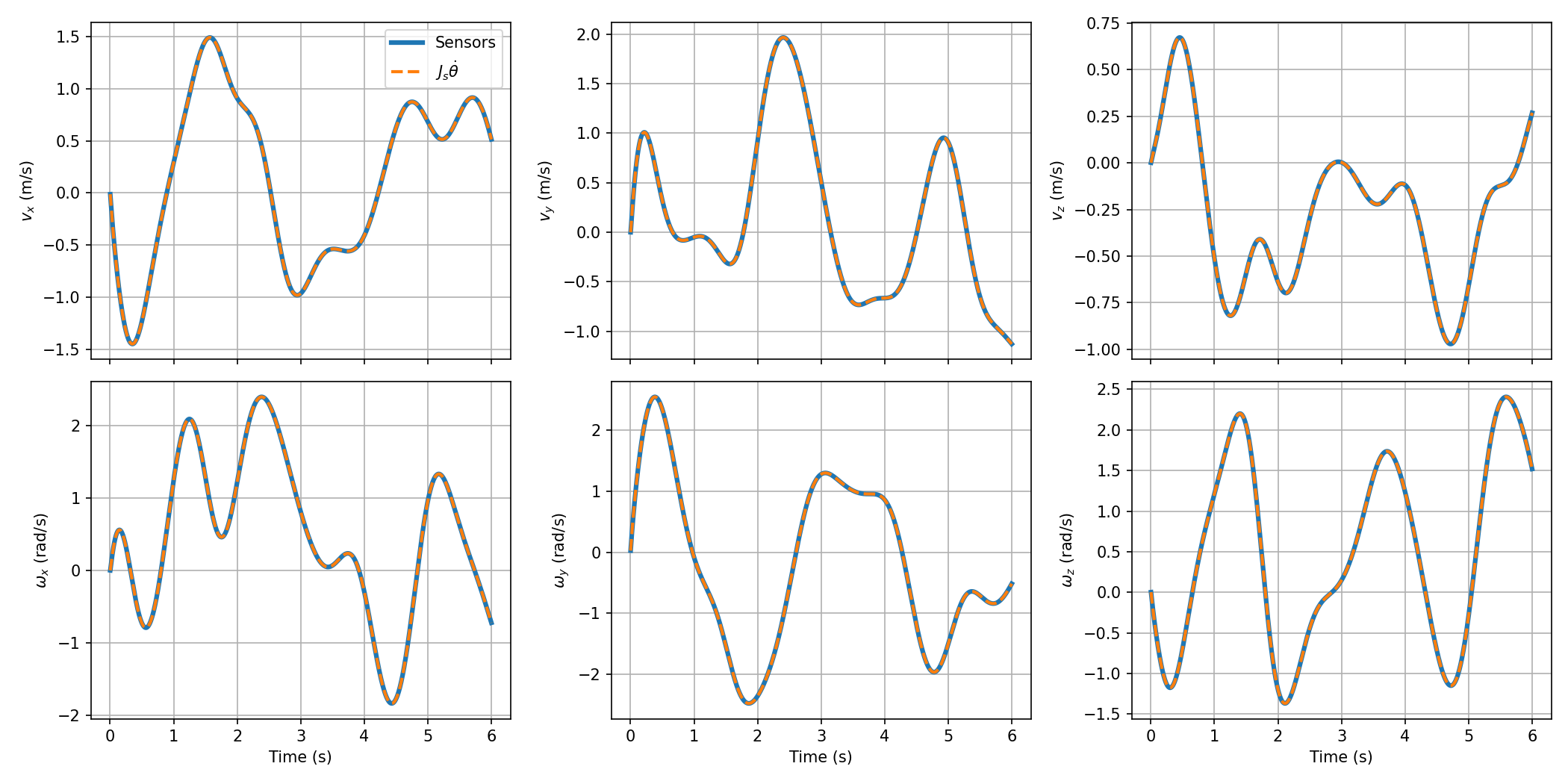
adjointis also used by the script to convert the sensor data. If both lines look wrong, checkadjointfirst.
Part B: Resolved-Rate Trajectories
Background
Part B moves the wrist along a straight line from \( g_{\text{start}} \) to \( g_{\text{end}} \) over a duration \( T \). The path is parameterized by \( s \in [0, 1] \):
\[p(s) = p_{\text{start}} + s \, (p_{\text{end}} - p_{\text{start}}), \qquad R(s) = R_{\text{start}} \exp\left( \ln\left( R_{\text{start}}^{\top} R_{\text{end}} \right) s \right),\]and the time scaling \( s(t) \) is a cubic with \( s(0) = 0 \), \( s(T) = 1 \), and \( \dot{s}(0) = \dot{s}(T) = 0 \).
The script samples the path at \( N + 1 \) evenly spaced times \( t_k \), with spacing \( \Delta t \), to get the waypoints \( g_k = g(s(t_k)) \). Resolved rate then finds the joint angles at each waypoint, starting from the known \( \theta_0 \):
\[\hat{\xi}_{s,k} = \frac{1}{\Delta t} \ln\left( g_{k+1} \, g_k^{-1} \right), \qquad \theta_{k+1} = \theta_k + \Delta t \, J_s(\theta_k)^{\dagger} \, \xi_{s,k} .\]The robot then tracks the joint angles \( \theta_k \), interpolated between waypoints.
Skeleton Code
Create trajectories.py with the following content. Your job is to fill in the parts marked TODO. twist_vector is given; it turns a \( 4 \times 4 \) twist matrix back into the vector \( (v, \omega) \).
import numpy as np
from scipy.linalg import expm, logm
from transforms import homogeneous
from kinematics import spatial_jacobian


def twist_vector(xi_hat):
    """Twist [v; omega] from its 4x4 twist matrix."""
    return np.array([xi_hat[0, 3], xi_hat[1, 3], xi_hat[2, 3],
                     xi_hat[2, 1], xi_hat[0, 2], xi_hat[1, 0]])


def time_scaling(t, T):
    """Cubic s(t) with s(0) = 0, s(T) = 1, and zero velocity at both ends."""
    t = min(max(t, 0.0), T)
    # TODO: evaluate the cubic time scaling at t
    return 0.0


def straight_line_path(g_start, g_end, s):
    """Pose at s along the straight-line path from g_start to g_end."""
    R_start, p_start = g_start[:3, :3], g_start[:3, 3]
    R_end, p_end = g_end[:3, :3], g_end[:3, 3]
    # TODO: position and orientation at s (wrap logm in np.real)
    p = p_start
    R = R_start
    return homogeneous(R, p)


def path_twist(g_now, g_next, dt):
    """Spatial twist that moves g_now to g_next in time dt."""
    # TODO: use logm and twist_vector (wrap logm in np.real)
    return np.zeros(6)


def resolved_rate_step(theta, xi, dt):
    """One resolved-rate update using the spatial Jacobian."""
    # TODO: use spatial_jacobian and np.linalg.pinv
    return theta
Running/Testing your Code
Create module2_path.py with the following content. Two settings at the top control the run:
METHOD = "resolved-rate"uses your resolved-rate update.METHOD = "joint"instead moves along a straight line in joint space, from \( \theta_{\text{start}} \) to \( \theta_{\text{end}} \), with the same time scaling.Nis the number of steps between waypoints.
import time
import mujoco
import mujoco.viewer
import numpy as np
import matplotlib
matplotlib.use("Agg")  # save the plot to a file instead of opening a window
import matplotlib.pyplot as plt
from kinematics import forward_kinematics_exponential
from trajectories import time_scaling, straight_line_path, path_twist, resolved_rate_step

METHOD = "resolved-rate"  # "resolved-rate" or "joint"
N = 20                    # number of steps between waypoints

m = mujoco.MjModel.from_xml_path("ur5e_model/scene.xml")
d = mujoco.MjData(m)
wrist = m.site("wrist").id

# Start and goal. The goal pose comes from a joint configuration so that the
# "joint" method has something to aim for; resolved rate only uses g_end.
theta_start = np.array([0, -np.pi/2, np.pi/2, -np.pi/2, -np.pi/2, 0])
theta_end = theta_start + np.array([1.5, 0.4, -0.6, 0.3, 0.4, 0.6])
g_start = forward_kinematics_exponential(theta_start)
g_end = forward_kinematics_exponential(theta_end)
T = 3.0               # duration of the motion (s)
duration = T + 1.0

# Waypoints along the straight-line path at evenly spaced times
t_k = np.linspace(0, T, N + 1)
dt = t_k[1] - t_k[0]
g_k = [straight_line_path(g_start, g_end, time_scaling(t, T)) for t in t_k]

# Joint angles at each waypoint
theta_k = [theta_start]
for k in range(N):
    if METHOD == "resolved-rate":
        xi = path_twist(g_k[k], g_k[k + 1], dt)
        theta_k.append(resolved_rate_step(theta_k[-1], xi, dt))
    else:  # straight line in joint space, with the same time scaling
        theta_k.append(theta_start + time_scaling(t_k[k + 1], T) * (theta_end - theta_start))
theta_k = np.array(theta_k)

def theta_desired(t):
    """Interpolate between the joint-angle waypoints."""
    return np.array([np.interp(t, t_k, theta_k[:, j]) for j in range(6)])

d.qpos[:6] = theta_start
times, p_actual = [], []

with mujoco.viewer.launch_passive(m, d) as viewer:
    # Green spheres: waypoints of the straight-line path
    for k, g in enumerate(g_k):
        mujoco.mjv_initGeom(viewer.user_scn.geoms[k], type=mujoco.mjtGeom.mjGEOM_SPHERE,
                            size=[0.015, 0, 0], pos=g[:3, 3], mat=np.eye(3).flatten(),
                            rgba=[0, 1, 0, 0.5])
    viewer.user_scn.ngeom = len(g_k)

    step = 0
    while viewer.is_running() and d.time < duration:
        step_start = time.time()

        # The UR5e motors are position servos: d.ctrl is the desired joint angle
        d.ctrl[:] = theta_desired(d.time)
        mujoco.mj_step(m, d)

        times.append(d.time)
        p_actual.append(d.site_xpos[wrist].copy())

        # Blue dots: where the wrist actually went
        if step % 25 == 0 and viewer.user_scn.ngeom < viewer.user_scn.maxgeom:
            mujoco.mjv_initGeom(viewer.user_scn.geoms[viewer.user_scn.ngeom],
                                type=mujoco.mjtGeom.mjGEOM_SPHERE, size=[0.006, 0, 0],
                                pos=d.site_xpos[wrist], mat=np.eye(3).flatten(),
                                rgba=[0, 0, 1, 1])
            viewer.user_scn.ngeom += 1
        step += 1

        viewer.sync()
        time.sleep(max(0, m.opt.timestep - (time.time() - step_start)))

# Compare three things against the straight line:
#   waypoints:   the desired poses g_k (on the line by construction)
#   result:      where the wrist would be at the planned joint angles theta_k
#   actual wrist: where the wrist went in the simulation
p_start, p_end = g_start[:3, 3], g_end[:3, 3]
direction = (p_end - p_start) / np.linalg.norm(p_end - p_start)
def distance_from_line(p):
    r = p - p_start
    return np.linalg.norm(r - (r @ direction) * direction)

p_waypoints = np.array([g[:3, 3] for g in g_k])
p_result = np.array([forward_kinematics_exponential(th)[:3, 3] for th in theta_k])
p_actual = np.array(p_actual)
result_label = "Resolved-rate result" if METHOD == "resolved-rate" else "Joint-space result"

print(f"Method: {METHOD}, N = {N}")
print("Wrist at the planned joint angles, largest distance from the line (m):",
      round(max(distance_from_line(p) for p in p_result), 4))
print("Wrist at the planned joint angles, final distance from the goal (m):",
      round(np.linalg.norm(p_result[-1] - p_end), 4))
print("Actual wrist, largest distance from the line (m):",
      round(max(distance_from_line(p) for p in p_actual), 4))

# Plot the path from above
fig, ax = plt.subplots(figsize=(7, 6))
ax.plot([p_start[0], p_end[0]], [p_start[1], p_end[1]], "k--", label="Straight line")
ax.plot(p_waypoints[:, 0], p_waypoints[:, 1], "o", color="tab:green", label="Waypoints $g_k$")
ax.plot(p_result[:, 0], p_result[:, 1], "s", color="tab:orange", markersize=5, label=result_label)
ax.plot(p_actual[:, 0], p_actual[:, 1], color="tab:blue", linewidth=2, label="Actual wrist")
ax.set_xlabel("x (m)")
ax.set_ylabel("y (m)")
ax.set_title(f"Wrist path (top view), {METHOD}, N = {N}")
ax.axis("equal")
ax.grid(True)
ax.legend()
fig.tight_layout()
name = f"module2_path_{METHOD}_N{N}.png"
fig.savefig(name, dpi=150)
print("Saved", name)
Then run it from your folder:
python module2_path.py
macOS: use
mjpythoninstead ofpythonto run any script that opens the viewer, e.g.mjpython module2_path.py.
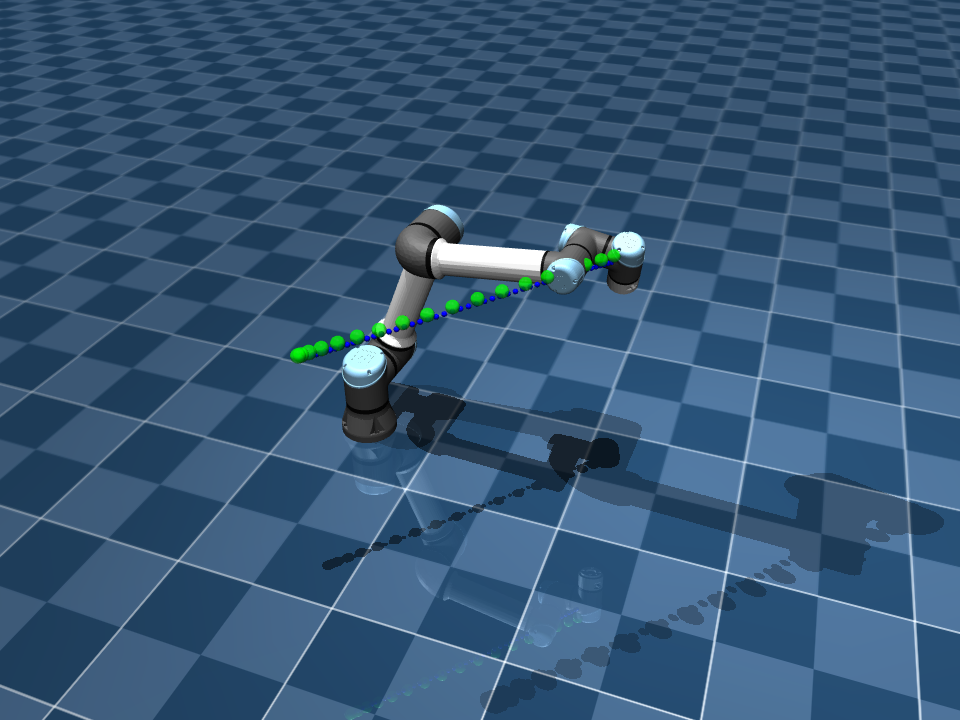
The green spheres are the waypoints of the straight-line path, and the blue dots show where the wrist actually went. If your code is correct, with METHOD = "resolved-rate" the blue dots stay close to the green spheres:
When the motion ends, the script saves a plot of the wrist path seen from above, named after the method and N (for example, module2_path_resolved-rate_N20.png). The plot compares three things:
- the waypoints \( g_k \) (green), which lie on the straight line by construction,
- the resolved-rate result (orange), which is where the wrist would be at the joint angles \( \theta_k \) from resolved rate, computed with your forward kinematics, and
- the actual wrist (blue), from the simulation.
If resolved rate were exact, the orange squares would sit on the green waypoints.
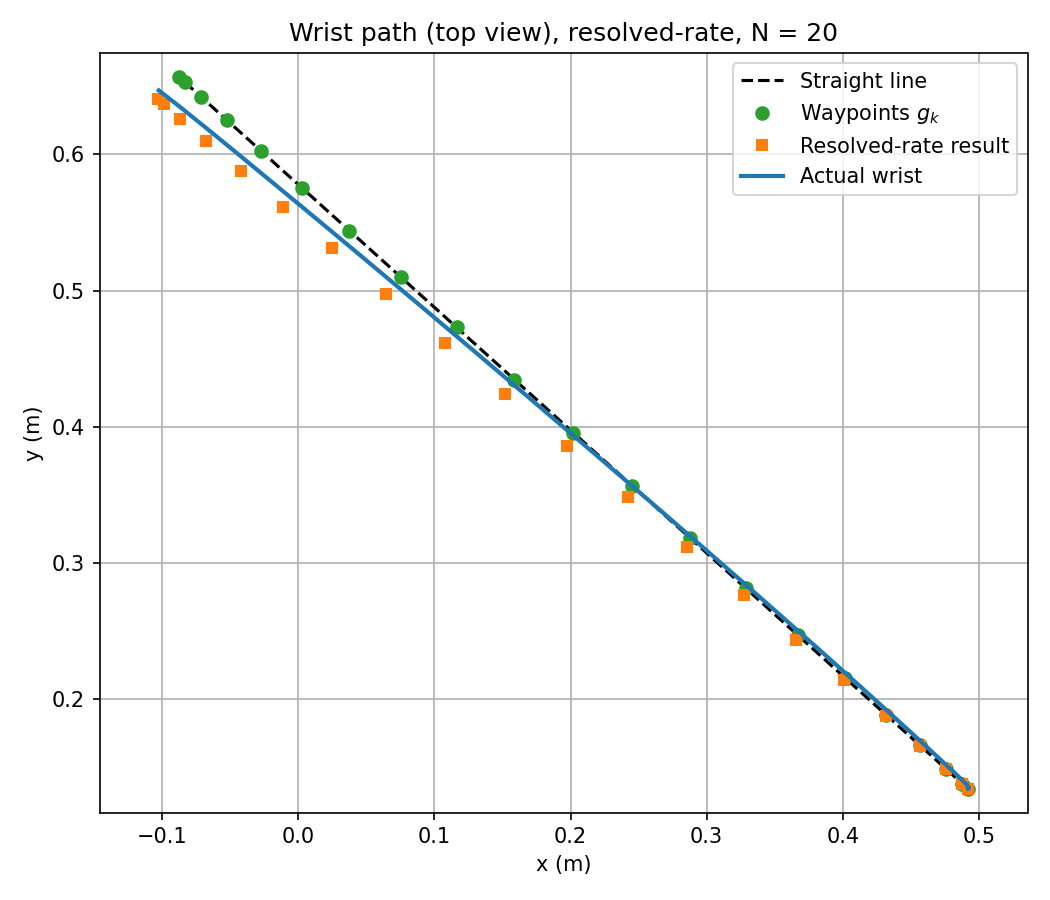
Next, run the script with a few values of N, such as 5, 20, and 100, and compare the plots. You can also set METHOD = "joint" to see the path that a straight line in joint space gives instead.
What to submit
Part A:
- The formulas you used to compute the spatial Jacobian (the adjoint and the columns \( \xi’_i \)).
- Your
module2_twist.pngplot.
Part B:
- Your plots for a few values of
N(for example, 5, 20, and 100). - An explanation of how the choice of
Naffects the drift of the resolved-rate result away from the waypoints. - A few sentences on how this drift could be improved, and what that other method would require.