Spatial and Body Velocity
This demo uses the one degree-of-freedom manipulator from Lecture 6 (Example 2.5 from MLS Chapter 2.4). Frame $A$ is fixed to the base, frame $B$ is attached to the end of the second link, and the robot rotates by $\theta$ about the vertical joint axis.
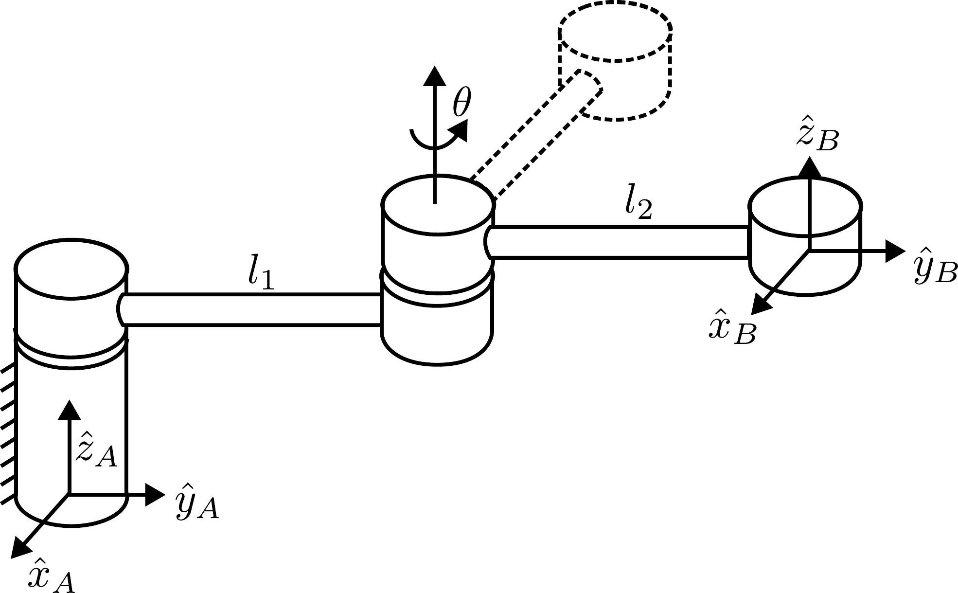
The configuration of frame $B$ relative to frame $A$ is:
\[g_{ab}(t) = \begin{bmatrix} R(t) & p(t) \\ 0 & 1 \end{bmatrix} = \begin{bmatrix} \cos\theta & -\sin\theta & -l_2 \sin\theta \\ \sin\theta & \cos\theta & l_1 + l_2 \cos\theta \\ 0 & 0 & 1 \end{bmatrix}\]The spatial and body velocities are computed from $g$ and its time derivative:
\[\hat{\xi}_s = \dot{g} g^{-1} \;\Rightarrow\; \begin{Bmatrix} v_s \\ \omega_s \end{Bmatrix} = \begin{Bmatrix} -\dot{R}R^{\top}p + \dot{p} \\ (\dot{R}R^{\top})^{\vee} \end{Bmatrix}, \qquad \hat{\xi}_b = g^{-1} \dot{g} \;\Rightarrow\; \begin{Bmatrix} v_b \\ \omega_b \end{Bmatrix} = \begin{Bmatrix} R^{\top}\dot{p} \\ (R^{\top}\dot{R})^{\vee} \end{Bmatrix}\]Interactive Demo
The robot is drawn from above, so $\hat{z}_A$ and $\hat{z}_B$ point out of the screen. Drag the $\theta$ slider to rotate the joint by hand, or press Play to rotate at a constant $\dot{\theta}$. The $l_1$ and $l_2$ sliders change the link lengths.
\(\dot{\theta}\) is estimated from how fast you drag the \(\theta\) slider \(\dot{\theta}\) is held constant (preset trajectory)
Current \(\dot{\theta}\): 0.00 rad/s
Spatial velocity
\(\omega_s =\) 0.00 \(= \dot{\theta}\)
\(v_s =\) 0.000.00 \(= \begin{bmatrix} l_1 \dot{\theta} \\ 0 \end{bmatrix}\)
Body velocity
\(\omega_b =\) 0.00 \(= \dot{\theta}\)
\(v_b =\) 0.000.00 \(= \begin{bmatrix} -l_2 \dot{\theta} \\ 0 \end{bmatrix}\)
For comparison: \(\dot{p}\)
\(\dot{p} =\) 0.000.00 \(= \begin{bmatrix} -l_2 \cos\theta \, \dot{\theta} \\ -l_2 \sin\theta \, \dot{\theta} \end{bmatrix}\)
What to Notice
- The velocities do not depend on $\theta$. For a fixed $\dot{\theta}$, $v_s$, $\omega_s$, $v_b$ and $\omega_b$ stay the same as the robot rotates. Compare this with $\dot{p}$, the velocity of $B$’s origin written in $A$ coordinates, which changes direction as $\theta$ changes.
- Spatial velocity ($v_s$, orange): imagine the rigid body extended far enough to reach the origin of $A$. $v_s$ is the velocity of the body point that is passing through $A$’s origin, written in $A$ coordinates. That point moves on the orange dashed circle of radius $l_1$ around the joint, so $v_s = l_1 \dot{\theta}$ along $\hat{x}_A$.
- Body velocity ($v_b$, blue): the velocity of $B$’s origin, written in $B$ coordinates. $B$’s origin moves on the blue dashed circle of radius $l_2$, always in the $-\hat{x}_B$ direction, so $v_b = -l_2 \dot{\theta}$ along $\hat{x}_B$.
- Angular velocity is $\dot{\theta}$ about $\hat{z}$ in both frames, since $\hat{z}_A$ and $\hat{z}_B$ always point the same way for this robot.