Inverse Kinematics with Geometric Approach
The geometric approach to inverse kinematics uses trigonometry to solve for the joint angles required to achieve a desired position. In particular, the approach leverages the law of cosines for the following triangle:
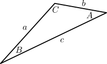
where the law of cosines gives us the equations:
\[A = \cos^{-1}\left(\frac{b^2 + c^2 - a^2}{2bc}\right), \quad B = \cos^{-1}\left(\frac{a^2 + c^2 - b^2}{2ac}\right)\]For our planar manipulator, we can obtain these side lengths using the desired end-effector position \((x_d, y_d)\) and the link lengths \((L_1, L_2, L_3)\). Note that we will assume a fixed wrist angle of zero for simplicity:
\[\begin{eqnarray} a &=& L_1 \nonumber \\ b &=& L_2 + L_3 \nonumber \\ c &=& \sqrt{x_d^2 + y_d^2} \nonumber \\ \end{eqnarray}\]Assuming that our zero configuration is with the robot along the x-axis, our diagrams corresponding to the “elbow-up” or “elbow-down” configurations are illustrated as follows:
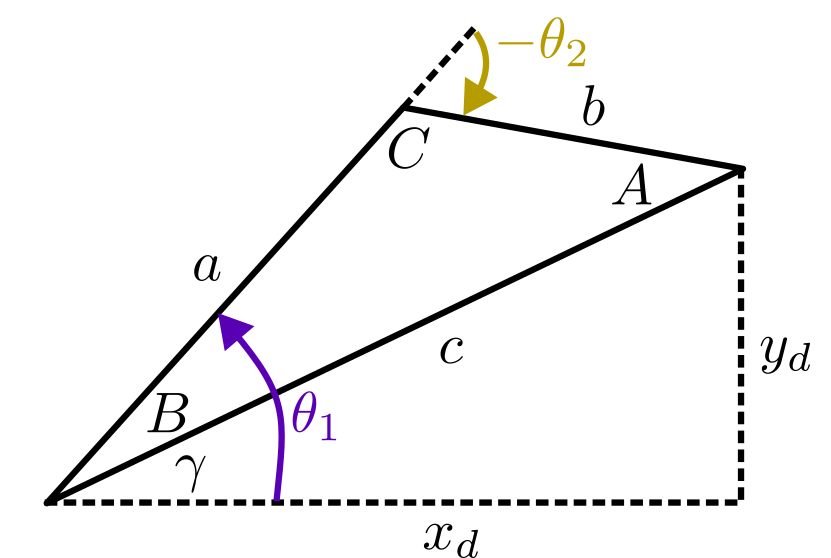
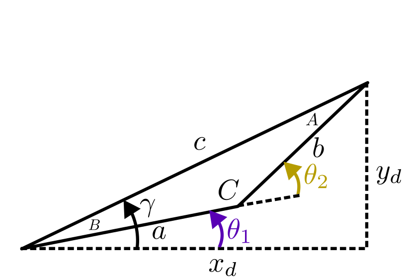
For any configuration, we can compute the angle \(\gamma\) using the two-input arctangent function:
\[\gamma = \mathrm{atan2}(y_d,x_d)\]Finally, based on the selected configuration, our joint angles are solved for as follows:
Elbow-Up Configuration:
\[\begin{eqnarray} \theta_1 &=& B + \gamma \nonumber \\ \theta_2 &=& C - \pi \nonumber \end{eqnarray}\]Elbow-Down Configuration:
\[\begin{eqnarray} \theta_1 &=& \gamma - B \\ \theta_2 &=& \pi - C \end{eqnarray}\]A demonstration of this approach is shown below for the “elbow-up” configuration: