The SO-101 Robot Arms
For this module, you will be designing and tracking a cubic spline trajectory on the SO-101 robot arm to perform a pick-and-place task.
Outline
- Assignment Part 1: Create a Cubic Spline Trajectory
- Assignment Part 2: Test in Simulation
- Assignment Part 3: Test on Hardware
- Optional Challenge - Straight Line Path in Task Space
- Submission Details
Assignment Part 1: Create a Cubic Spline Trajectory
To move between two joint configurations using a cubic spline, we will create a modified move_to_pose_cubic function. This function should mostly use the same code as in move_to_pose but with the addition of the following:
- Define the cubic spline coefficients based on the starting and desired joint positions, as well as the duration of the movement. For now we will assume zero starting and ending velocities.
# Cubic coefficients stored in a dictionary similar to starting_position a0 = starting_position a1 = {joint: ?? for joint in starting_position} a2 = {joint: ?? for joint in starting_position} a3 = {joint: ?? for joint in starting_position} - Create a helper function to evaluate the cubic spline at a given time
tfor each joint. This time should be clipped to remain in the range[0, duration].
def cubic_interpolation(t, joint): tlim = min(max(t, 0), duration) pos = a0[joint] + a1[joint]*tlim + a2[joint]*(tlim**2) + a3[joint]*(tlim**3) return pos - Update the position_dict in the control loop to use the cubic spline evaluation instead of linear interpolation.
 # Interpolate each joint
 position_dict = {}
 for joint in desired_position:
     p0 = starting_position[joint]
     pf = desired_position[joint]
     position_dict[joint] = cubic_interpolation(t, joint)
Optional: Adding Velocity Control
To make our tracking even better, we should add velocity commands using the cubic splines. This takes a decent bit of code change in MuJoCo, but is simpler to implement on hardware. In general, the important code changes are the following:
    def cubic_interpolation(t, joint):
        tlim = min(max(t, 0), duration)
        pos = a0[joint] + a1[joint]*tlim + a2[joint]*(tlim**2) + a3[joint]*(tlim**3)
        vel = a1[joint] + 2*a2[joint]*tlim + 3*a3[joint]*(tlim**2)
        return pos, vel
with the control loop updated to:
    # Interpolate each joint
    position_dict = {}
    velocity_dict = {}
    for joint in desired_position:
        position_dict[joint], velocity_dict[joint] = cubic_interpolation(t, joint)
Then, in MuJoCo, we need to update the send_position_command function to also accept velocity commands
def send_position_command(d, position_dict, velocity_dict=None):
    pos = convert_to_list(position_dict)
    vel = convert_to_list(velocity_dict) if velocity_dict is not None else [0.0]*6
    d.ctrl = np.hstack([pos, vel])
and the model (so101_new_calib.xml) to accept velocity inputs for the motors.
  <actuator>
    <position class="sts3215" kp="50" kv="2" name="shoulder_pan" joint="shoulder_pan" forcerange="-10 10" ctrlrange="-1.91986 1.91986"/>
    <position class="sts3215" kp="50" kv="2" name="shoulder_lift" joint="shoulder_lift" forcerange="-10 10" ctrlrange="-1.74533 1.74533"/>
    <position class="sts3215" kp="50" kv="2" name="elbow_flex" joint="elbow_flex" forcerange="-10 10" ctrlrange="-1.69 1.69"/>
    <position class="sts3215" kp="50" kv="2" name="wrist_flex" joint="wrist_flex" forcerange="-10 10" ctrlrange="-1.65806 1.65806"/>
    <position class="sts3215" kp="50" kv="2" name="wrist_roll" joint="wrist_roll" forcerange="-10 10" ctrlrange="-2.74385 2.84121"/>
    <position class="sts3215" kp="50" kv="2" name="gripper" joint="gripper" forcerange="-10 10" ctrlrange="-0.17453 1.74533"/>
    <velocity class="sts3215" kv="10" name="shoulder_pan_vel" joint="shoulder_pan" forcerange="-10 10" ctrlrange="-200 200"/>
    <velocity class="sts3215" kv="10" name="shoulder_lift_vel" joint="shoulder_lift" forcerange="-10 10" ctrlrange="-200 200"/>
    <velocity class="sts3215" kv="10" name="elbow_flex_vel" joint="elbow_flex" forcerange="-10 10" ctrlrange="-200 200"/>
    <velocity class="sts3215" kv="10" name="wrist_flex_vel" joint="wrist_flex" forcerange="-10 10" ctrlrange="-200 200"/>
    <velocity class="sts3215" kv="10" name="wrist_roll_vel" joint="wrist_roll" forcerange="-10 10" ctrlrange="-200 200"/>
    <velocity class="sts3215" kv="10" name="gripper_vel" joint="gripper" forcerange="-10 10" ctrlrange="-200 200"/>
  </actuator>
For some very strange reason burried in the depths of MuJoCo, the
<default>class does not work for setting the Kd gains. For this reason, you need to list the gains within the<actuator>section explicitly as shown in the code block above. Note that I’ve changed these gains from our previous labs to have improved tracking.
On hardware, velocity commmands are not currently supported by the LeRobot hardware code, so we will still only send position commands to the robot.
Assignment Part 2: Test in Simulation
Before moving to hardware, you can first test the cubic spline trajectory in MuJoCo. To do this, try executing the following script:
import time
import mujoco
import mujoco.viewer
from so101_mujoco_utils import set_initial_pose, send_position_command, move_to_pose_cubic
from so101_inverse_kinematics import get_inverse_kinematics
import numpy as np


m = mujoco.MjModel.from_xml_path('model/scene_with_velocity.xml')
d = mujoco.MjData(m)

size_block = 0.0285 #in meters (1.125 inches)
pos1 = [0.25, 0.1, size_block/2]
pos2 = [0.25, -0.1, size_block/2]
config1 = get_inverse_kinematics(pos1)
config2 = get_inverse_kinematics(pos2)

# Helper Function to show a cube at a given position and orientation
def show_cube(viewer, position, orientation, geom_num=0, halfwidth=0.013):
    color = np.random.rand(3).tolist() + [1]  # Random RGB, alpha=0.2
    mujoco.mjv_initGeom(
      viewer.user_scn.geoms[geom_num],
      type=mujoco.mjtGeom.mjGEOM_BOX,
      size=[halfwidth, halfwidth, halfwidth],
      pos=position,
      mat=orientation.flatten(),
      rgba=color
    )
    viewer.user_scn.ngeom += 1
    viewer.sync()
    return

# Initial joint configuration at start of simulation
initial_config = {
    'shoulder_pan': 0.0,
    'shoulder_lift': 0.0,
    'elbow_flex': 0.00,
    'wrist_flex': 0.0,
    'wrist_roll': 0.0,
    'gripper': 0
}
set_initial_pose(d, initial_config)
send_position_command(d, initial_config)

# Start simulation with mujoco viewer
with mujoco.viewer.launch_passive(m, d) as viewer:

  # Show the target positions
  show_cube(viewer, pos1, np.eye(3), geom_num=0)
  show_cube(viewer, pos2, np.eye(3), geom_num=1)

  # Wait for one second before the simulation starts
  time.sleep(1.0)

  # Cubic spline to first configuration
  move_to_pose_direct(m, d, viewer, initial_config, config1, 2.0)
  hold_position(m, d, viewer, 1.0)

  # Cubic spline to second configuration
  move_to_pose_direct(m, d, viewer, config1, config2, 2.0)
  hold_position(m, d, viewer, 1.0)

  # Cubic spline to initial configuration
  move_to_pose_direct(m, d, viewer, config2, initial_config, 2.0)
  hold_position(m, d, viewer, 1.0)
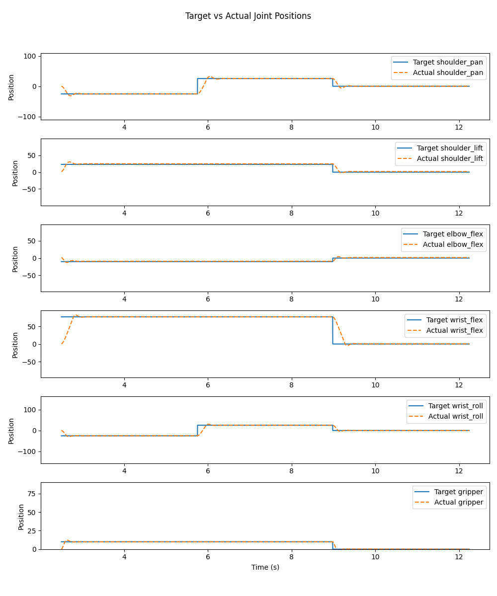
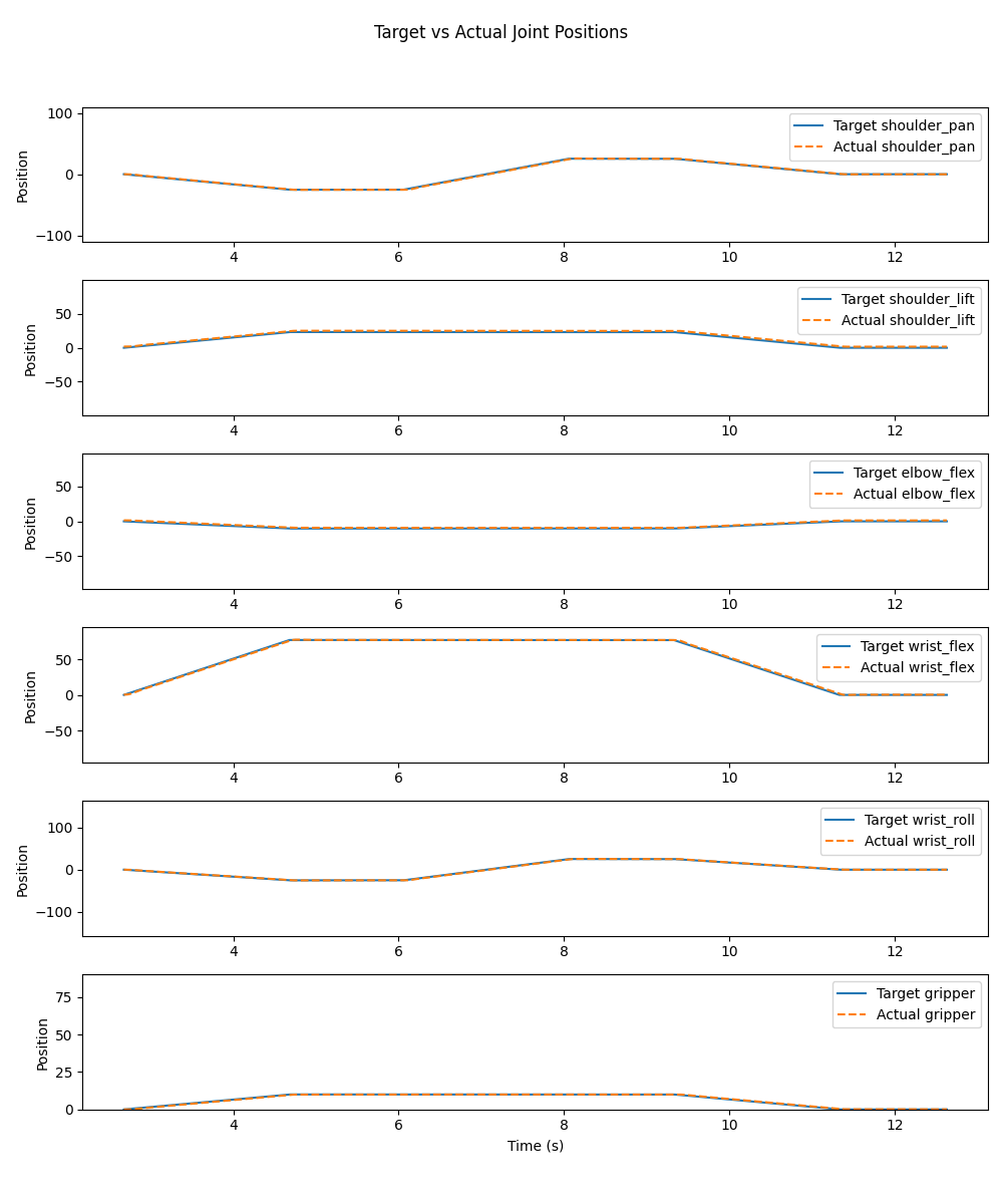
The tracking associated with each of these videos is the following.
Assignment Part 3: Test on Hardware
Lastly, implement your cubic spline trajectory using the move_to_pose_cubic function on hardware. This will use the same code as in simulation, but now the positions will be sent as follows. You can implement this for just a single motion (like the video above for simulation) or try implementing it for the stacking blocks task from Lab 8.
Adding velocity commands on hardware is not currently supported by the LeRobot hardware code, so we will only be sending position commands to the robot. I’m still exploring this a bit to see if it’s possible, so if you discover any workarounds please let me know!
Optional Challenge - Straight Line Path in Task Space
If you are looking for an additional challenge, try implementing a straight line in task space between two desired positions. What we’ve been doing so far has implemented a straight line in joint space. But if instead we want a straight line path in task space, we have two options:
- Implement IK in each control loop to track a straight line path in the end-effector position. If you want to still use a cubic spline for this method, you will need to implement the cubic spline for time rescaling as discussed in Lecture 21.
- Implement resolved-rate trajectory design (more complicated than necessary since we have closed-form solutions for IK).
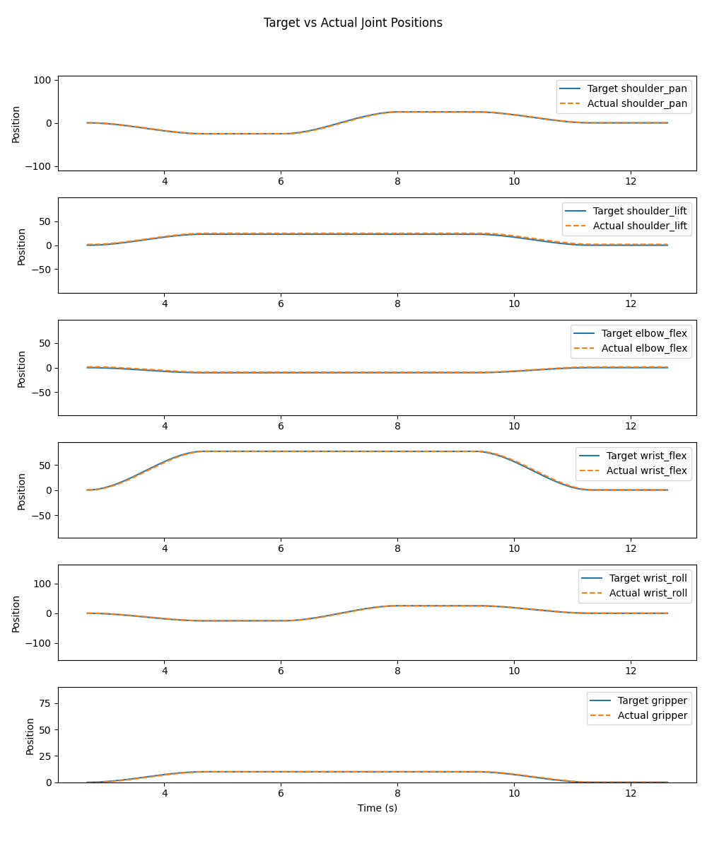
Below shows the results from Method 1 (using cubic splines for time rescaling with IK in the control loop tracking a straight-line path in task space). You will be implementing Method 2 for the homework component of Assignment 9.
Submission Details
As usual, please include a writeup in your homework submission about the lab this week. Describe the difference you saw between the cubic spline trajectory and the linear interpolation trajectory on both simulation and hardware. Discuss the tracking performance, smoothness of motion, and any other observations you had.
Additionally, please either show the TAs during lab TA office hours a demonstration of your cubic spline trajectory on hardware. Or, if this is not possible, please email a video of your robot (preferably a youtube link) to Prof Tucker with the TAs cc’ed.