The SO-101 Robot Arms

For this module, we will be writing code to calculate the inverse kinematics for our SO-101 robot arms using a geometric approach. We will then repeat the same “Pick and Place” maneuver from Lab 6 but without needing pre-determined joint configurations. For this week we will be focusing on testing our inverse kinematics solution in simulation only, and then you will be asked to implement a pick and place demonstration on hardware next week.

Outline

• Assignment Part 0: Redo the Forward Kinematics
• Assignment Part 1: Derive the Inverse Kinematics
  • 1a) Set up Inverse Kinematics Functions
  • 1b) Solve for $\theta_1$
  • 1c) Solve for Desired Position of the Wrist Frame
  • 1d) Solve for $\theta_2$ and $\theta_3$
  • 1e) Solve for $\theta_4$
  • 1f) Solve for $\theta_5$
• Assignment Part 2: Test the Inverse Kinematics
  • 2a) Understand the Workspace
  • 2b) Test Random Target Positions
• Submission Details

Assignment Part 0: Redo the Forward Kinematics

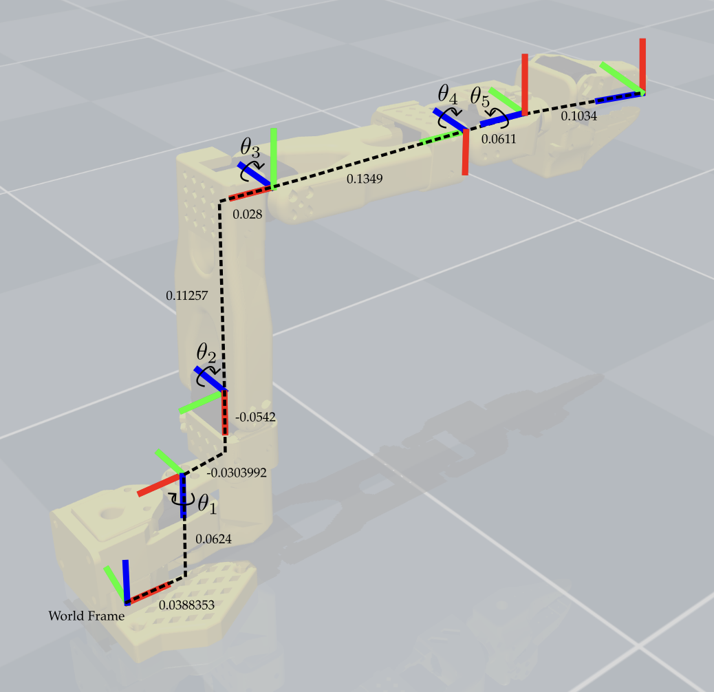
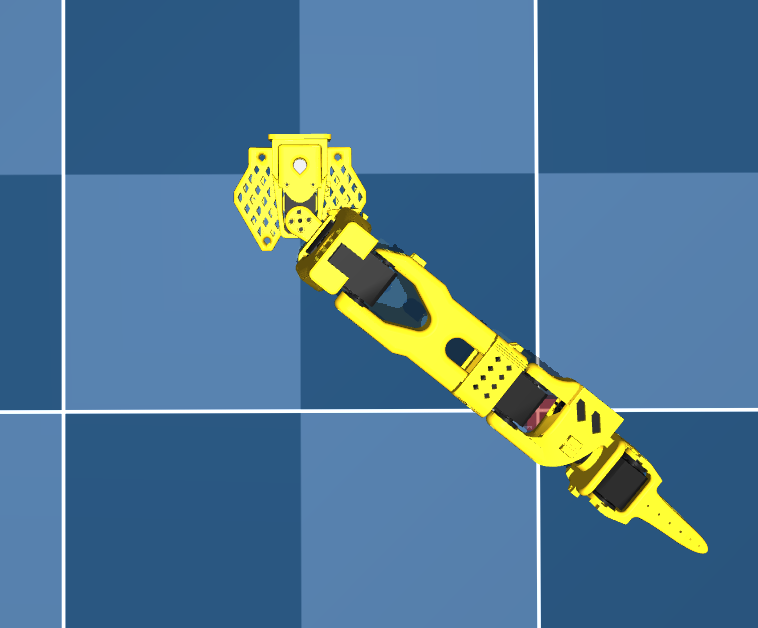
To make the inverse kinematics derivation easier, I recommend redoing the forward kinematics so that the tool frame is in the same orientation as the wrist frame when it’s pointed straight down. This can be done by modifying the orientation of the tool frame to match the diagram below:

Assignment Part 1: Derive the Inverse Kinematics

1a) Set up Inverse Kinematics Functions

First, write a helper script named so101_inverse_kinematics.py that takes in a desired tool frame position and orientation and returns the corresponding joint configuration. We will populate this script with all zeros to start:

def get_inverse_kinematics(target_position, target_orientation):
    "Geometric appraoch specific to the so-101 arms"
    
    # Initialize the joint configuration dictionary
    joint_config = {
        'shoulder_pan': 0.0,
        'shoulder_lift': 0.0,
        'elbow_flex': 0.0,
        'wrist_flex': 0.0,
        'wrist_roll': 0.0,
        'gripper': 0.0
    }

Then, we will write a test simulation script named run_mujoco_simulation_testIK.py that will use this function to move the robot to a desired position. The following code provides a starting point for this script:

import time
import mujoco
import mujoco.viewer
from so101_mujoco_utils import set_initial_pose, send_position_command, move_to_pose, hold_position
from so101_inverse_kinematics import get_inverse_kinematics
import numpy as np

m = mujoco.MjModel.from_xml_path('model/scene.xml')
d = mujoco.MjData(m)

# Helper Function to show a cube at a given position and orientation
def show_cube(viewer, position, orientation, geom_num=0, halfwidth=0.013):
    mujoco.mjv_initGeom(
        viewer.user_scn.geoms[geom_num],
        type=mujoco.mjtGeom.mjGEOM_BOX, 
        size=[halfwidth, halfwidth, halfwidth],                 
        pos=position,                         
        mat=orientation.flatten(),              
        rgba=[1, 0, 0, 0.2]                           
    )
    viewer.user_scn.ngeom = 1
    viewer.sync()
    return
  
# Initial joint configuration at start of simulation
initial_config = {
    'shoulder_pan': 0.0,
    'shoulder_lift': 0.0,
    'elbow_flex': 0.00,
    'wrist_flex': 0.0,
    'wrist_roll': 0.0,
    'gripper': 0          
}
set_initial_pose(d, initial_config)
send_position_command(d, initial_config)

# Start simulation with mujoco viewer
with mujoco.viewer.launch_passive(m, d) as viewer:
  
  # Specify the desired position of the cube to be picked up
  desired_position = [0.2, 0.2, 0.014]

  # Add a cylinder as a site for visualization
  show_cube(viewer, desired_position, np.eye(3))
  
  # First send the robot to a higher position with the gripper open
  joint_configuration = get_inverse_kinematics(temp_desired_position, viewer)
  move_to_pose(m, d, viewer, joint_configuration, 1.0)
  
  # Hold position for 10 seconds
  hold_position(m, d, viewer, joint_configuration, 10.0)

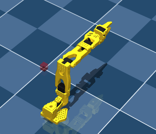
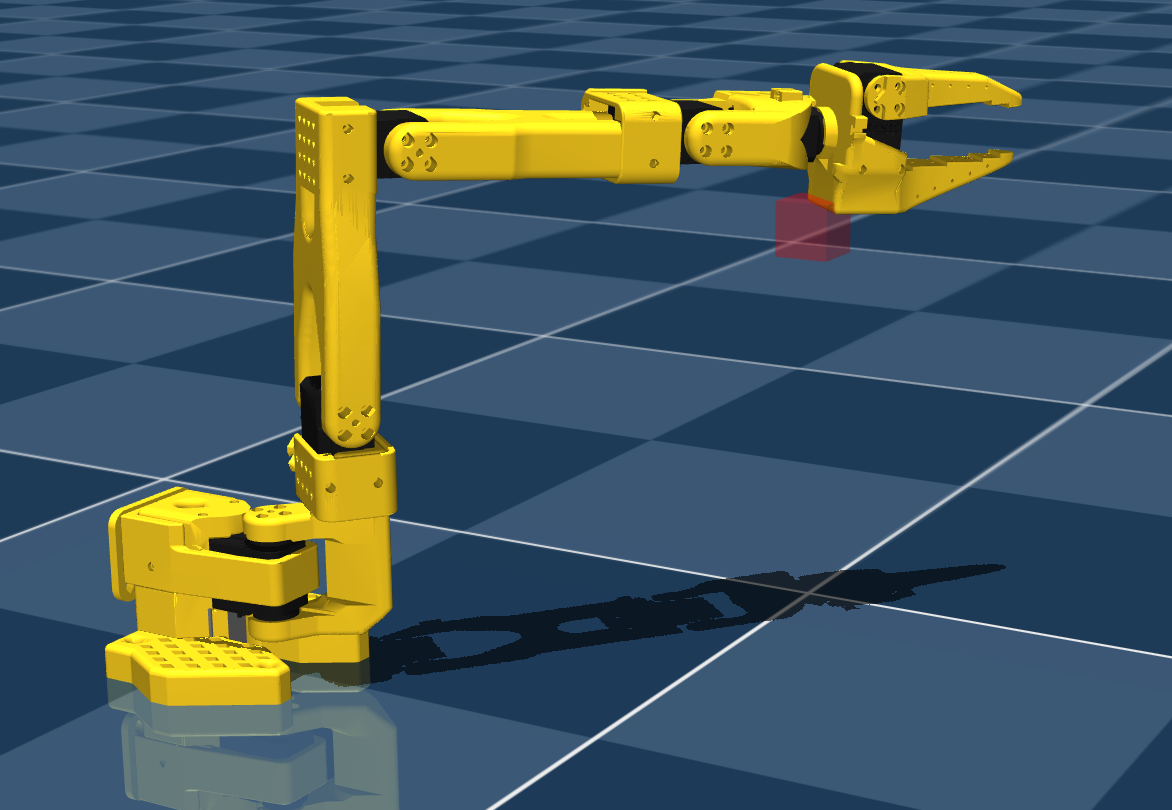
If you run this script now, the robot will not move since the inverse kinematics function is not yet implemented, but you should see the following:

1b) Solve for $\theta_1$

We can break down the geometric appraoch in our case to first solve for $\theta_1$. To do this, we can project the desired end-effector position onto the ground plane (i.e., the x-y plane) and use trigonometry to solve for $\theta_1$ using the diagram below:

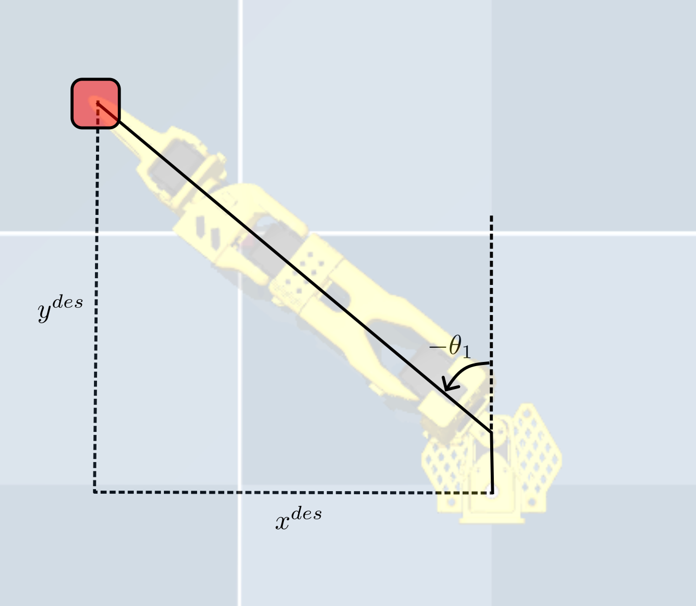
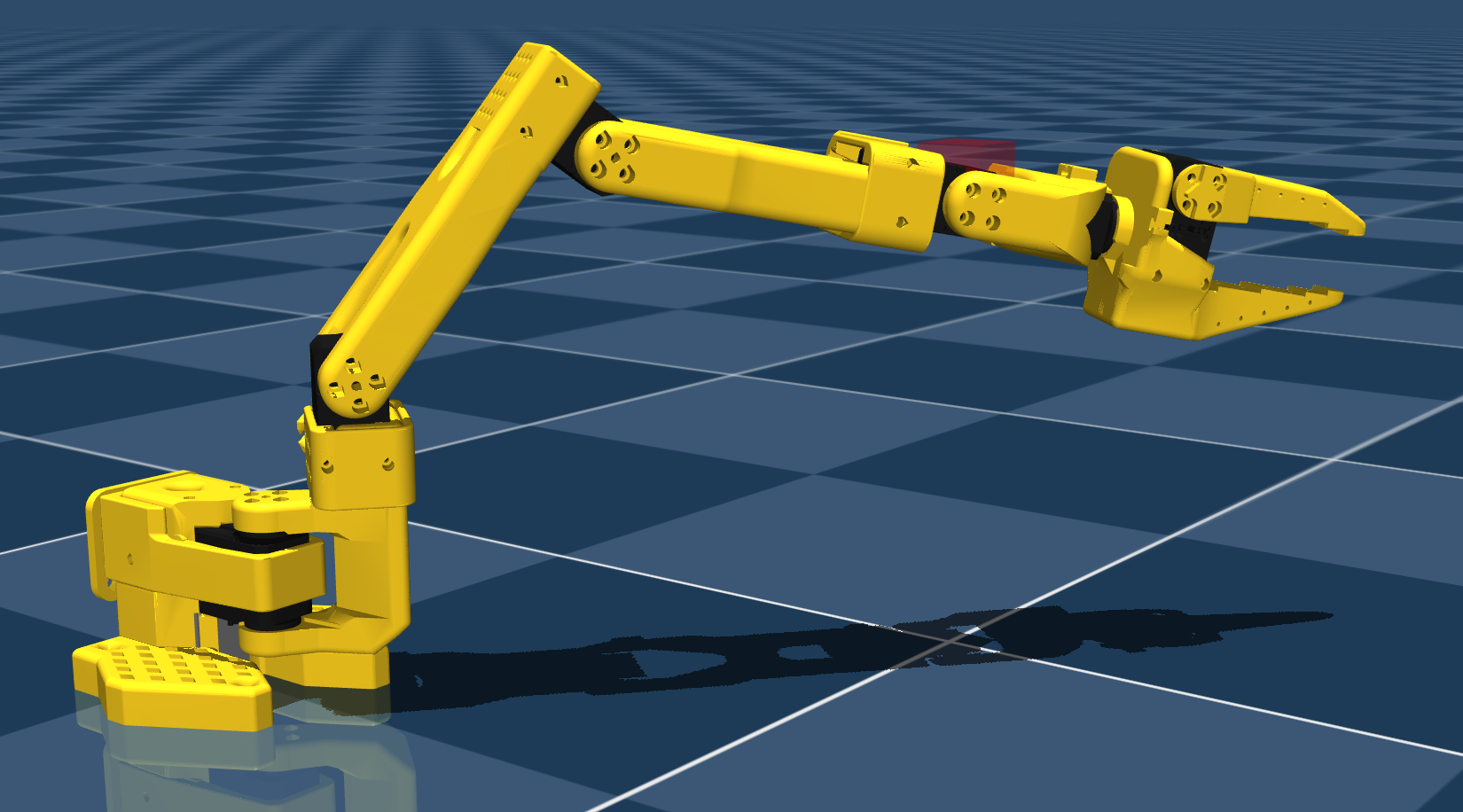
If you do this correctly, you should see the manipulator arm line up with the position of the block.

Be careful, if you do not account for the frame’s offset in the x-axis correctly, the robot will not line up exactly with the block!

Incorrect Alignment (Bad)

Correct Alignment (Good)

1c) Solve for Desired Position of the Wrist Frame

Once $\theta_1$ is solved, the next step is to solve for the desired position of the wrist frame (i.e., the center of the frame attached at joint 4) assuming that we want to grasp the object from above (i.e., assuming that the desired end-effector orientation will only change with respect to the z-axis). This will be done by writing a helper function in your so101_inverse_kinematics.py script that computes the desired wrist position based on the desired end-effector position using the equation

\[g_{w4} = g_{wt} g_{4t}^{-1}\]

where $g_{wt}$ is the desired target position in the world frame, and $g_{4t}$ is computed as $g_{4t} = g_{45}(0) g_{5t}$ using the same helper functions as in our forward kinematics from Lab 6.

The following code snippet provides a starting point for this function:

def get_wrist_flex_position(target_position):
    gwt = ?
    g4t = ?
    gw4 = gwt @ np.linalg.inv(g4t)
    wrist_flex_position = ?
    wrist_flex_orientation = ?
    return wrist_flex_position, wrist_flex_orientation

Which will then be evaluated in your main inverse kinematics function as follows:

    target_wrist_position = get_wrist_flex_position(target_position)

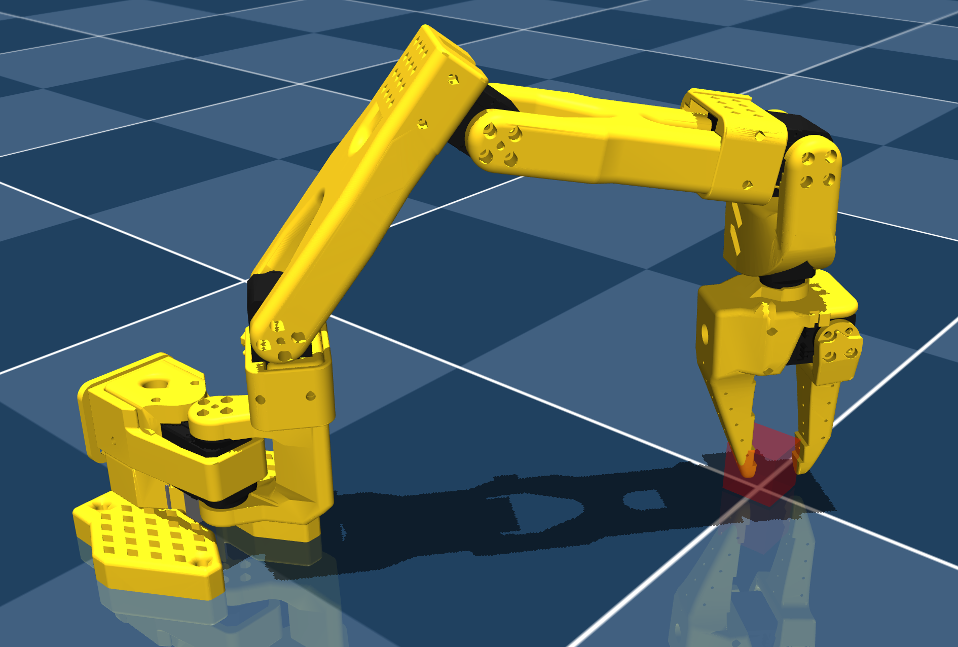
You can test whether or not this worked properly by displaying a cube at the calculated wrist position in your simulation script. If done correctly, you should see the following:

1d) Solve for $\theta_2$ and $\theta_3$

Now your job is to solve for $\theta_2$ and $\theta_3$ to position the wrist frame at the desired wrist position calculated in the previous step. You can use a similar geometric approach as in Lab 6 to solve for these two joint angles. To do this, I recommend drawing out the manipulator arm in the plane and drawing the triangle formed between the frames of joint 1, 2, and 3. You should then label the lengths of each side of the triangle and use the law of cosines to solve for the two joint angles.

If done correctly, you should see the following result in simulation:

1e) Solve for $\theta_4$

Next, solve for $\theta_4$ in order to position the end-effector such that $z_{tool}$ is aligned with the world z-axis. You can do this by first calculating the current orientation of the wrist frame using forward kinematics, and then calculating the difference in orientation between the current wrist frame and the desired wrist frame. Since we are only concerned with aligning the z-axes, you can project both z-axes onto the x-y plane and calculate the angle between them. This angle will correspond to $\theta_4$.

This can similarly be done by drawing a vertical line on your triangle diagram from part d and solving for the corresponding angle.

If done correctly, you should see the following result in simulation:

1f) Solve for $\theta_5$

The last step is to solve for $\theta_5$ in order to align the end-effector orientation with the desired target orientation. You can either do this using trigonometry or we can make the simple observation that the only axes influencing the rotation about the z-axis are $\theta_1$ and $\theta_5$. Therefore, if we assume that our desired orientation is zero, we can use $ \theta_5 = -\theta_1 $.

However, since $\theta_5$ has the opposite joint axis as $\theta_1$, we need to negate this value again to get the correct joint angle. Therefore, our final expression is: \(\theta_5 = \theta_1\).

If done correctly, you should see the following result in simulation: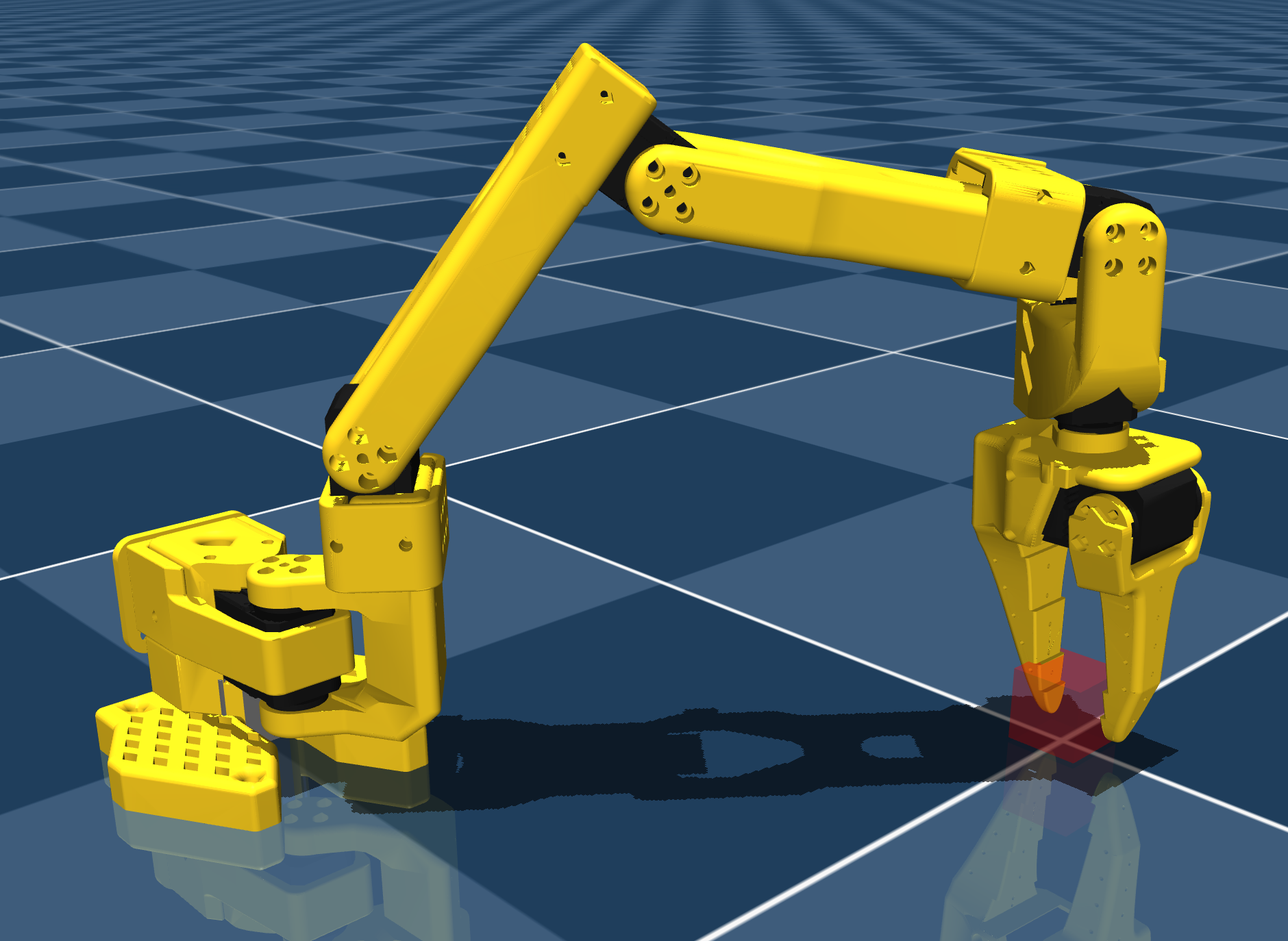

Assignment Part 2: Test the Inverse Kinematics

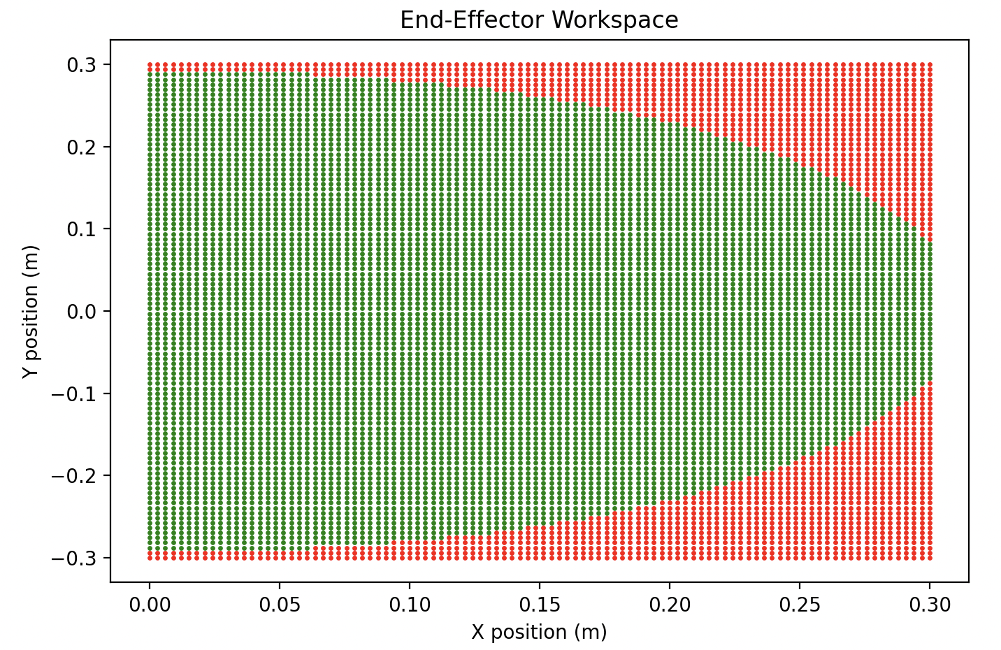
To test your inverse kinematics solution, we will modify the run_mujoco_simulation_testIK.py script to move the robot to various random desired target positions. This will first require understanding the workspace of the SO-101 robot arm with a vertical grasp.

2a) Understand the Workspace

We can obtain the workspace by looping through target positions and analyzing whether or not the inverse kinematics solution returns NaN values for the joint angles. If the solution returns NaN, then the target position is outside of the robot’s workspace. You do not need to code this up on your own, but if you’d like to better understand workspace analysis than I recommend trying it for yourself. Otherwise, you can refer to the following plot for your analysis:

2b) Test Random Target Positions

Once you understand the workspace, modify your run_mujoco_simulation_testIK.py script to randomly sample target positions within the workspace and move the robot to those positions using your inverse kinematics solution. You should use the following code snippet within your script to do this:

# Helper function to obtain random target position and yaw (rotation around the z-axis) from a given range 
def get_random_position():
    x_pos_range = [X, X] #taken from workspace analysis
    y_pos_range = [X, X] #taken from workspace analysis
    yaw_range = [0, np.pi/2] #anything beyond 0 to 90 degrees is redundant due to symmetry of the cube
    x = np.random.uniform(x_pos_range[0], x_pos_range[1])
    y = np.random.uniform(y_pos_range[0], y_pos_range[1])
    yaw = np.random.uniform(yaw_range[0], yaw_range[1])
    return [x, y, 0.014], yaw

# Start simulation with mujoco viewer
with mujoco.viewer.launch_passive(m, d) as viewer:
  
  # Pause for 10 seconds in order to make screen recording easier
  time.sleep(10) 
  
  while viewer.is_running():
    
    for i in range(5):
      desired_position, desired_yaw = get_random_position()
      desired_orientation = np.eye(3)

      # Add a cylinder as a site for visualization
      show_cube(viewer, desired_position, desired_orientation)
      
      # Get the inverse kinematics solution
      joint_configuration = get_inverse_kinematics(desired_position, desired_orientation)

      # Move the robot to the desired pose
      move_to_pose(m, d, viewer, joint_configuration, 1.0)
      
      # Hold for two seconds for easy visualization
      hold_position(m, d, viewer, joint_configuration, 2.0)

Your final video submission should look something like this:

Submission Details

Please show your simulation to one of the TAs during lab office hours. If this is not possible, you may also email a video to Prof. Tucker with the TAs cc-ed. For full credit, each group member must also submit a writeup of how they completed the geometric inverse kinematics solution, including diagrams with labeled lengths and angles for $\theta_1$, $\theta_2$, and $\theta_3$.