Final project for Caltech Robotics course ME133a
As my final project for the Caltech robotics course, ME 133a, I developed a custom MATLAB software to simulate three different serial chain robots using Denavit-Hartenberg parameters. These parameters follow a strict set of rules that specify the location and orientation of each link frame for a rigid robotic device. Each frame corresponds to one of the joint axes. Once the Denavit-Hartenberg (D-H) parameters are defined, the transformation between each frame can be calculated using the D-H parameters. The forward kinematics of the mechanism can then be calculated using all of the frame transformations. The Guided User Interface (GUI) outlined in this report visualizes a robot as defined by its D-H parameters and calculates the forward kinematics and spatial manipulator Jacobian of the robot given the final joint variables.
Project Summary
The main outcome of this project is a kinematics and visualization software. The inputs of the software are the Denavit-Hartenberg parameteres as defined by the user. Then using these Denavit-Hartenberg parameters, the software creates a visual representation of the specified robot and calculates the forward kinematics and spatial manipulator Jacobian. A figure of the initial GUI screen can be seen below.
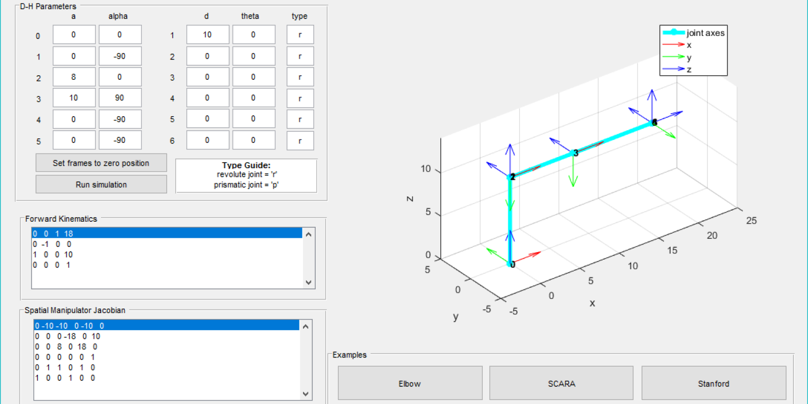
Initial GUI Output
The motivation for this project was to create a software that made it easier to visualize the relationship between Denavit-Hartenverg parameters and the associated robotic mechanism. The software can also be used to erify the validity of Denavit-Hartenberg parameters derived for a specific robot with known geometry. The software also makes it faster to obtain the forward kinematics and spatial manipulator Jacobian for different final configurations of robotic mechanisms.
The scope of this project covers Denavit-Hartenberg parameters, the modified transformmation matrix, forward kinematics, and the spatial manipulator Jacobian. These principles are implemented into software using MATLAB and guided user interface.
Project Details
The visualization of the robotic mechanism was obtained from the transformation matrix of each frame individually. The calculation of all of the transformation matrices occurs in the subfunction “modtransform”. The function uses the modified Denavit-Hartenberg frame transformation equation as shown below.
\[g_{i/i+1} = \begin{bmatrix} cos{\theta_{i+1}} & -sin{\theta_{i+1}} & 0 & a_i \\\ sin{\theta_{i+1}}cos{\alpha_i} & cos{\theta_{i+1}}cos{\alpha_i} & -sin{\alpha_{i}} & -d_isin{\alpha_i} \\\ sin{\theta_{i+1}}sin{\alpha_i} & cos{\theta_{i+1}}sin{\alpha_i} & cos{\alpha_{i}} & d_icos{\alpha_i} \\\ 0 & 0 & 0 & 1 \end{bmatrix}\]The values for $\alpha$ and $\theta$ are both entered in degrees for ease of use with the GUI. For a robot with N Degrees of Freedom, the modtransform function would output N+1 transformation matrices. The first N transformation matrices are for each of the joint frames from the stationary frame. The last transformation matrix is the total transformation matrix from the stationary frame to the tool frame. A transformation matrix is defined in general as the following.
\[g_{AB} = \begin{bmatrix} R_{AB} & \overline{d_{AB}} \\\ \overline{0}^T & 1 \end{bmatrix}\]Thus, for the \(i^{th}\) transformation matrix of the first N transformation matrices, the transformation matrix gives us the location and orientation of the \(i^{th}\) frame. The location of the frame is given by \(\overline{d_{AB}}\) and the rotation of the frame coordinates are given by the columns of \(R_{AB}\) where each column is a vector for each frame coordinate.
Forward Kinematics
The forward kinematics of the entire mechanism was calculated using the transformation matrix of each frame as shown in the following equation.
\[g_{st}(\theta) = g_{l_0l_1}(\theta_1)g_{l_1l_2}(\theta_2) \dots g_{l_5l_6}(\theta_6)g_{l_6l_t}\]For the purposes of this software, the tool frame was assumed to be the same as the last frame.This multiplication results in a final matrix as shown below.
\[g_{st} = \begin{bmatrix} R_{st} & \overline{d_{st}} \\\ \overline{0}^T & 1 \end{bmatrix}\]Where \(R_{st}\) is the rotation matrix of the tool frame coordinates from the stationary frame coordinates and \(\overline{d_{st}}\) is the displacement of the tool frame from the stationary frame. This matrix was output to the GUI in the “Forward Kinematics” panel. The user can vary the inputs for the joint variables and analyze how each change in joint variable effects the forward kinematics of the entire mechanism. The forward kinematics can be verified in the following software screenshot.
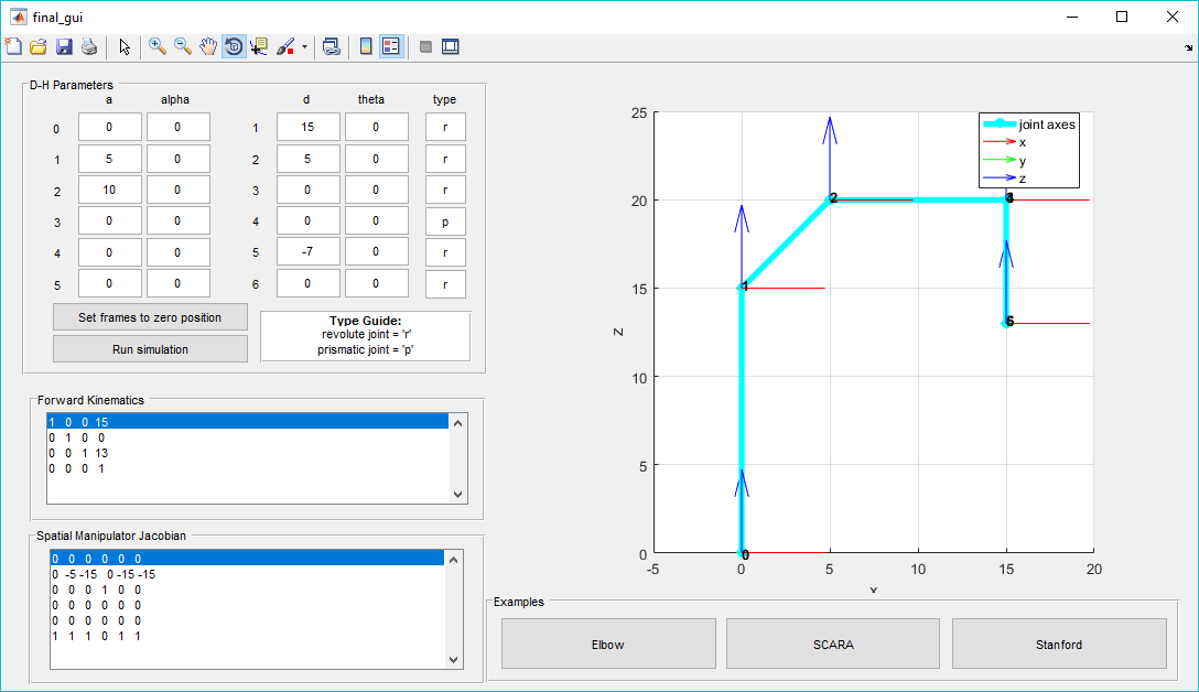
Verification of Forward Kinematics of SCARA manipulator at Zero Position
The forward kinematics indicates that the tool frame has zero rotation and a displacement of 15 units in the x-direction, 0 in the y-direction, and 13 in the z-direction.This results can be visually verified from the visual representation of the manipulator.
Spatial Manipulator Jacobian
The spatial manipulator Jacobian illustrates the twist for each joint axis in the mechanism. The \(i^{th}\) column of the Jacobian corresponds to the \(i^{th}\) joint axis twist. For a revolute joint, the joint twist was calculated as follows.
\[\xi_i = \begin{bmatrix} -\omega_i \times q_i \\\ \omega_i \end{bmatrix}\]Where \(\omega_i\) is the direction of the \(i^{th}\) joint axis and $q_i$ is the location of the \(i^{th}\) joint frame from the stationary frame. Both \(\omega_i\) and \(q_i\) are in reference to the stationary frame.
For a prismatic joint, since the pitch of the joint is infinite, the joint twist is calculated as follows. \(\xi_i = \begin{bmatrix} \omega_i \\\ \overline{0} \end{bmatrix}\)
The Jacobian for the entire mechanism is output to the GUI in the “Spatial Manipulator Jacobian” panel. This output also allows users to investigate how different joint parameters influence the Jacobian.