This project was my final project for the Caltech robotics course 133b.

Bug algorithms are very effective strategies for robotic path planning when the robot has a global goal but only local information about the environment is known. The benefits of bug algorithms is that the behaviors are simple and they are straightforward to implement. A disadvantage of bug algorithms is that it assumes perfect positioning and sensing. This problem could be diminished by using LIDAR data to keep track of the robots position instead of relying on wheel odometry and IMU sensors. As shown in Lab 3, odometry obtained from LIDAR data is much more accurate than wheel odometry or IMU integration.

In class, we learned about three bug algorithms: Bug I, Bug II, and Tangent Bug. For this project, I chose to implement the Tangent Bug algorithm in a MATLAB simulation environment.The Tangent Bug algorithm uses a finite range sensor to collect information about obstacles in the environment. In my simulation, the range sensor was assumed to be a LIDAR sensor. The Tangent Bug algorithm was selected because it provides the most “natural” and “intuitive” path to the goal. However, it is slightly more complicated than both Bug I and Bug II.

Project Summary

The main outcome of this project is a a graphical user interface (GUI) that demonstrates the Tangent Bug algorithm for seven different environments. Several supporting codes are used in this GUI.

The motivation for this project was to implement the Tangent Bug algorithm using LIDAR data. Even though this implementation is in a simulation environment. The algorithm does not use any information about the obstacles other than their intersection points with the simulated LIDAR beams. Thus, in theory this code could be used seamlessly with hardware to obtain the same results. However, the MATLAB simulation assumes that the robot is a point robot, so the desired [x,y] coordinates of the robot are directly commanded in simulation. In practice, an additional code would be needed to translate the desired coordinates into wheel velocities.

Project Details

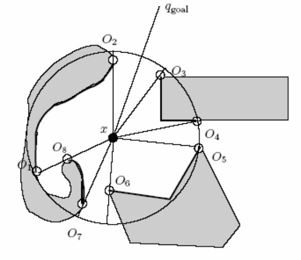
The basic idea of the Tangent Bug algorithm is that it uses both motion-to-goal and boundary following behaviors to reach a desired goal. The motion-to-goal behavior is commanded as long as there is no blocking obstacle or if the blocking obstacle does not increase the heuristic distance. The heuristic distance is calculated using the following equation.

where \(O_i\) is an edge point of a continuous segment of an obstacle as obtained from LIDAR data. A visual representation of these endpoints can be seen below.

Boundary following mode is commanded when the heuristic distance increases. The bug them remains in Boundary following mode until \(d_{reach} < d_{followed}\). The value \(d_{followed}\) is the shortest distance between the sensed boundary and the goal. The value \(d_{reach}\) is the shortest distance between the blocking obstacle and the goal.If there is no blocking obstacle, \(d_{reach}\) is the distance between the robot and the goal.

Algorithmic breakdown

Motion to Goal (While the heuristic distance is decreasing or remaining the same)

1. Compute Lidar Data
2. Move toward the obstacle
3. Terminate if the goal is reached

Boundary Following (While \(d_{reach} \geq d_{followed}\))

1. Update the Lidar data, \(d_{reach}\), and \(d_{followed}\)
2. Terminate if a complete cycle is completed (goal is unreachable)
3. Terminate if the goal is reached

Example Environments

The Tangent Bug algorithm can be used with any environment. To best demonstrate this implementation of the algorithm, seven different environments were created and included as options in the GUI.